tikatuwq: Water Quality Indices and Temporal Trends

Introduction

This vignette focuses on the methods implemented in tikatuwq for computing water quality indices and analyzing temporal trends. We cover:

Water Quality Index (IQA/WQI) calculation methods
Trophic State Index (IET) for lakes and reservoirs
Temporal trend analysis using robust and parametric methods
Parameter-specific analysis tools

Water Quality Index (IQA/WQI)

Method overview

The IQA combines sub-indices (Qi) for individual parameters using weighted arithmetic mean. The sub-indices are obtained by piecewise-linear interpolation over approximate curves (CETESB/NSF style).

library(tikatuwq)
data("wq_demo", package = "tikatuwq")

Default parameters and weights

The default IQA implementation uses 9 parameters with standard weights:

# Default weights
default_weights <- c(
  od = 0.17,
  coliformes = 0.15,
  dbo = 0.10,
  nt_total = 0.10,
  p_total = 0.10,
  turbidez = 0.08,
  tds = 0.08,
  pH = 0.12,
  temperatura = 0.10
)

# Check sum equals 1
sum(default_weights)
#> [1] 1

Computing IQA

# Compute IQA with default settings
df_iqa <- iqa(wq_demo, na_rm = TRUE)

# View results
cols_show <- intersect(c("ponto", "IQA", "IQA_status"), names(df_iqa))
head(df_iqa[, cols_show, drop = FALSE])
#> # A tibble: 6 × 3
#>   ponto         IQA IQA_status
#>   <chr>       <dbl> <ord>     
#> 1 FBS-BRH-250  89.8 Boa       
#> 2 FBS-BRH-250  93.1 Otima     
#> 3 FBS-BRH-250  92.2 Otima     
#> 4 FBS-BRH-250  87.6 Boa       
#> 5 FBS-BRH-250  95.7 Otima     
#> 6 FBS-BRH-300  89.3 Boa

# Distribution
hist(df_iqa$IQA, breaks = 10, main = "IQA Distribution", xlab = "IQA")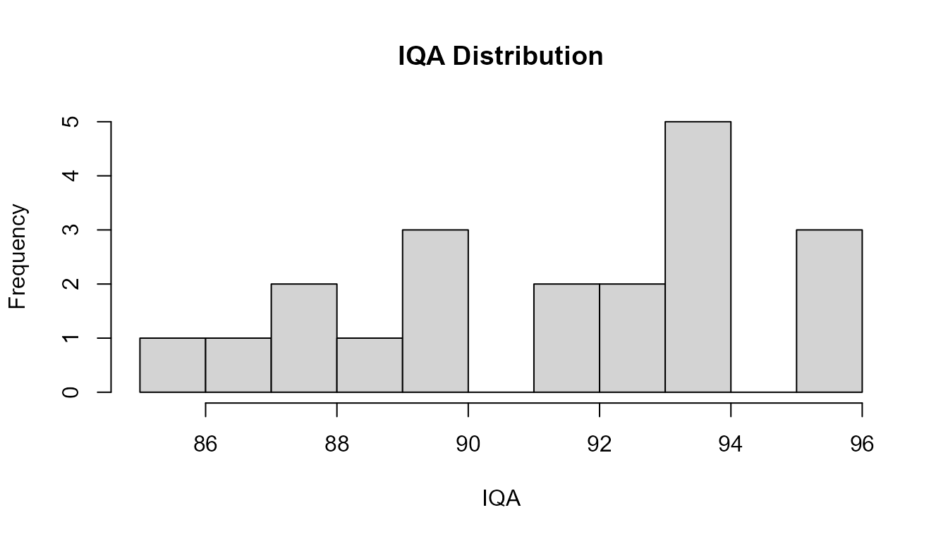

Figure generated by tikatuwq package

Handling missing parameters

When na_rm = TRUE, weights are rescaled per row to use only available parameters:

# Example with missing parameters
df_missing <- wq_demo
df_missing$tds <- NULL  # Remove one parameter

df_iqa_missing <- iqa(df_missing, na_rm = TRUE)
head(df_iqa_missing$IQA)
#> [1] 91.89265 95.23563 94.27265 89.02090 98.18742 91.06328

Custom weights

You can provide custom weights:

# Custom weights (must sum to 1)
custom_weights <- c(
  od = 0.20,
  coliformes = 0.20,
  dbo = 0.10,
  nt_total = 0.10,
  p_total = 0.10,
  turbidez = 0.10,
  tds = 0.10,
  pH = 0.05,
  temperatura = 0.05
)

df_iqa_custom <- iqa(wq_demo, pesos = custom_weights, na_rm = TRUE)
cols_show2 <- intersect(c("IQA", "IQA_status"), names(df_iqa_custom))
head(df_iqa_custom[, cols_show2, drop = FALSE])
#> # A tibble: 6 × 2
#>     IQA IQA_status
#>   <dbl> <ord>     
#> 1  92.4 Otima     
#> 2  96.0 Otima     
#> 3  95.2 Otima     
#> 4  89.5 Boa       
#> 5  99.1 Otima     
#> 6  92.9 Otima

Classification

The IQA values are automatically classified into qualitative categories:

# Classification function
classify_iqa(c(15, 40, 65, 80, 95))
#> [1] Muito ruim Ruim       Regular    Boa        Otima     
#> Levels: Muito ruim < Ruim < Regular < Boa < Otima

# English labels
classify_iqa(c(15, 40, 65, 80, 95), locale = "en")
#> [1] Very Poor Poor      Fair      Good      Excellent
#> Levels: Very Poor < Poor < Fair < Good < Excellent

# Distribution in demo data
table(df_iqa$IQA_status)
#> 
#> Muito ruim       Ruim    Regular        Boa      Otima 
#>          0          0          0          8         12

Trophic State Index (IET)

Carlson IET

For lentic systems, the Carlson Trophic State Index uses Secchi depth, chlorophyll-a, and total phosphorus:

# Example dataset with required parameters
# df_lake <- data.frame(
#   ponto = c("L1", "L2"),
#   secchi = c(2.5, 1.0),  # meters
#   clorofila = c(5, 20),  # ug/L
#   p_total = c(0.02, 0.10)  # mg/L (converted to ug/L internally)
# )
# 
# iet_carlson(df_lake, .keep_ids = TRUE)

The function automatically: - Converts p_total (mg/L) to tp (ug/L) if needed - Accepts aliases (sd for secchi, chla for clorofila) - Returns TSI values with classification

Lamparelli IET

Similar to Carlson but with different equations and thresholds:

# iet_lamparelli(df_lake, .keep_ids = TRUE)

Temporal Trend Analysis

Single parameter trend

The trend_param() function computes Theil-Sen slope and Spearman correlation:

# Add temporal structure to demo data
df_temporal <- wq_demo
df_temporal$data <- as.Date("2025-01-01") + seq_len(nrow(df_temporal)) - 1

# Compute trend for turbidity
trend_result <- trend_param(df_temporal, param = "turbidez")

print(trend_result)
#>        rio       ponto    param n   date_min   date_max days_span
#> 1 BURANHEM FBS-BRH-250 turbidez 5 2025-01-01 2025-01-05         4
#> 2 BURANHEM FBS-BRH-300 turbidez 5 2025-01-06 2025-01-10         4
#> 3 BURANHEM FBS-BRH-450 turbidez 5 2025-01-11 2025-01-15         4
#> 4 BURANHEM FBS-BRH-950 turbidez 5 2025-01-16 2025-01-20         4
#>   slope_per_year intercept rho_spearman p_value      trend pct_change_period
#> 1             NA        NA           NA      NA indefinido                NA
#> 2             NA        NA           NA      NA indefinido                NA
#> 3             NA        NA           NA      NA indefinido                NA
#> 4             NA        NA           NA      NA indefinido                NA

The result includes: - slope: Theil-Sen slope - p_value: Spearman correlation p-value - trend: classification (increasing, decreasing, stable)

Plotting trends

library(ggplot2)

# Plot with trend line
p_trend <- plot_trend(df_temporal, param = "turbidez", method = "theilsen")
print(p_trend)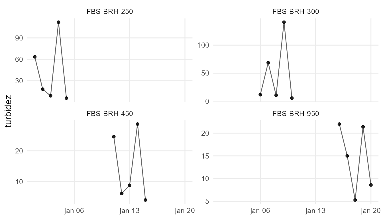

Figure generated by tikatuwq package


# With LOESS smoothing
p_loess <- plot_trend(df_temporal, param = "turbidez", method = "loess")
print(p_loess)

Figure generated by tikatuwq package

Multiple parameters

Use param_trend_multi() to analyze trends across multiple parameters:

# Trends for multiple parameters
params <- c("turbidez", "od", "dbo")
trends_multi <- param_trend_multi(df_temporal, parametros = params)

print(trends_multi)
#> # A tibble: 12 × 7
#>    rio      ponto           slope p_value       r2     n parametro
#>    <chr>    <chr>           <dbl>   <dbl>    <dbl> <int> <chr>    
#>  1 BURANHEM FBS-BRH-250 -2.17e+ 0  0.904  5.66e- 3     5 turbidez 
#>  2 BURANHEM FBS-BRH-300  6.04e+ 0  0.793  2.67e- 2     5 turbidez 
#>  3 BURANHEM FBS-BRH-450 -1.86e+ 0  0.674  6.69e- 2     5 turbidez 
#>  4 BURANHEM FBS-BRH-950 -2.04e+ 0  0.468  1.86e- 1     5 turbidez 
#>  5 BURANHEM FBS-BRH-250  2.54e- 1  0.286  3.58e- 1     5 od       
#>  6 BURANHEM FBS-BRH-300  2.20e- 1  0.253  4.00e- 1     5 od       
#>  7 BURANHEM FBS-BRH-450 -4.43e- 1  0.199  4.74e- 1     5 od       
#>  8 BURANHEM FBS-BRH-950 -5.85e- 1  0.478  1.79e- 1     5 od       
#>  9 BURANHEM FBS-BRH-250  2.91e-14  1.000  1.04e-26     5 dbo      
#> 10 BURANHEM FBS-BRH-300 -9.00e- 1  0.0577 7.50e- 1     5 dbo      
#> 11 BURANHEM FBS-BRH-450 -6   e- 1  0.182  5.00e- 1     5 dbo      
#> 12 BURANHEM FBS-BRH-950  1.99e-16  0.182  5.00e- 1     5 dbo

Parameter-specific Analysis

Summary statistics

# Summary for one parameter
summary_turb <- param_summary(df_temporal, parametro = "turbidez")
print(summary_turb)
#> # A tibble: 4 × 8
#>   rio      ponto           n  mean    sd   min median   max
#>   <chr>    <chr>       <int> <dbl> <dbl> <dbl>  <dbl> <dbl>
#> 1 BURANHEM FBS-BRH-250     5  41.7 45.6    5.8   18.3 112  
#> 2 BURANHEM FBS-BRH-300     5  47.4 58.4    5.4   11.4 141  
#> 3 BURANHEM FBS-BRH-450     5  14.4 11.4    4      8.8  28.7
#> 4 BURANHEM FBS-BRH-950     5  14.5  7.48   5.3   15    22

# Multi-parameter summary
summary_multi <- param_summary_multi(df_temporal, parametros = c("turbidez", "od", "dbo"))
print(summary_multi)
#> # A tibble: 12 × 9
#>    rio      ponto           n  mean     sd   min median    max parametro
#>    <chr>    <chr>       <int> <dbl>  <dbl> <dbl>  <dbl>  <dbl> <chr>    
#>  1 BURANHEM FBS-BRH-250     5 41.7  45.6    5.8   18.3  112    turbidez 
#>  2 BURANHEM FBS-BRH-300     5 47.4  58.4    5.4   11.4  141    turbidez 
#>  3 BURANHEM FBS-BRH-450     5 14.4  11.4    4      8.8   28.7  turbidez 
#>  4 BURANHEM FBS-BRH-950     5 14.5   7.48   5.3   15     22    turbidez 
#>  5 BURANHEM FBS-BRH-250     5  6.44  0.671  5.96   6.13   7.58 od       
#>  6 BURANHEM FBS-BRH-300     5  6.84  0.550  6.19   6.7    7.51 od       
#>  7 BURANHEM FBS-BRH-450     5  6.42  1.02   5.59   6.05   8.19 od       
#>  8 BURANHEM FBS-BRH-950     5  6.91  2.19   4.91   6.1   10.6  od       
#>  9 BURANHEM FBS-BRH-250     5  3.2   0.447  3      3      4    dbo      
#> 10 BURANHEM FBS-BRH-300     5  4.2   1.64   3      4      7    dbo      
#> 11 BURANHEM FBS-BRH-450     5  3.6   1.34   3      3      6    dbo      
#> 12 BURANHEM FBS-BRH-950     5  3     0      3      3      3    dbo

Parameter plots

# Single parameter plot
p1 <- param_plot(df_temporal, parametro = "turbidez")
print(p1)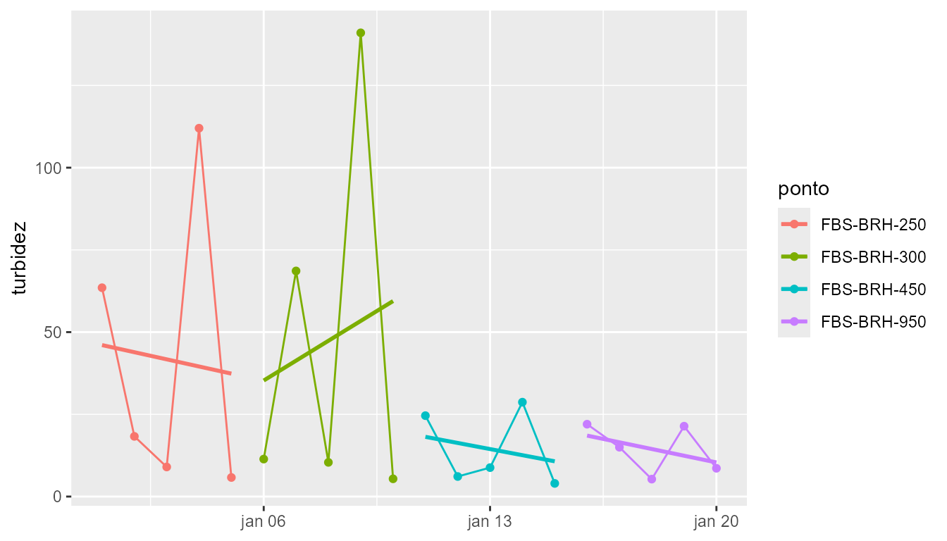

Figure generated by tikatuwq package


# Multi-parameter plot
p2 <- param_plot_multi(df_temporal, parametros = c("turbidez", "od", "dbo"))
print(p2)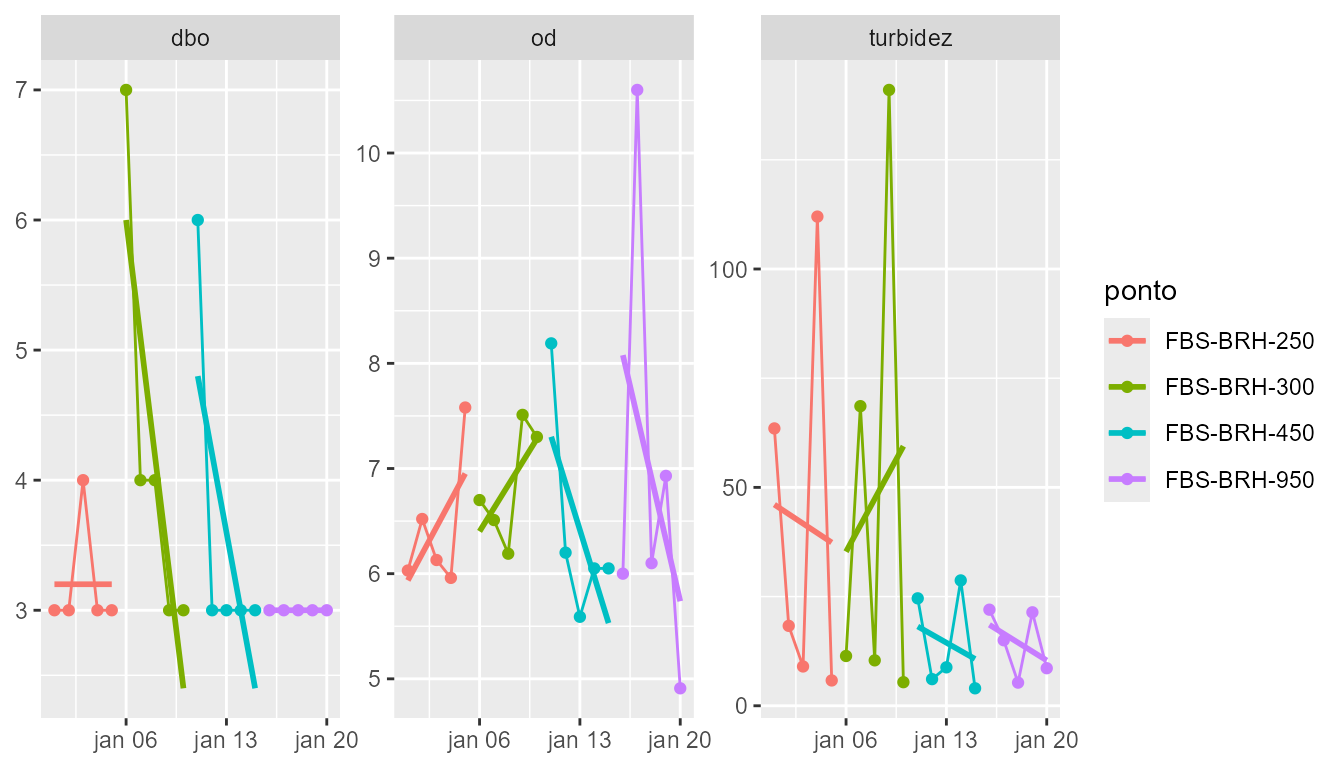

Figure generated by tikatuwq package

Statistical Methods

Theil-Sen estimator

The Theil-Sen method is robust to outliers:

# Theil-Sen computes median of all pairwise slopes
# For data with outliers, it is more reliable than OLS
# Used by default in trend_param() and plot_trend()

Spearman correlation

Non-parametric test for monotonic trends:

# Spearman correlation tests for monotonic relationship
# Does not assume linearity
# p-value indicates significance of trend

Best Practices

Choosing parameters for IQA

Include all 9 default parameters when possible
Use na_rm = TRUE if some parameters are missing
Adjust weights only if you have domain knowledge

Handling censored values

Use nd_policy = "ld2" (default) for conservative estimates
Consider nd_policy = "na" if censored values should not influence results
Document your choice in reports

Trend analysis

Use Theil-Sen for robust estimates with outliers
Require at least 4 observations per group for reliable trends
Consider seasonal effects when analyzing temporal data

Units consistency

Ensure all parameters use standard units (mg/L, NTU, etc.)
Use clean_units() to convert if needed
Document unit conversions in methodology sections

References

Carlson, R. E. (1977). A trophic state index for lakes. Limnology and Oceanography, 22(2), 361-369.
Lamparelli, M. C. (2004). Graus de trofia em corpos d’agua do estado de Sao Paulo: avaliacao dos metodos de monitoramento. Tese de Doutorado, Universidade de Sao Paulo.
CETESB. (2021). Aguas superficiais: indice de qualidade das aguas (IQA). Companhia Ambiental do Estado de Sao Paulo.

Summary

This vignette covered:

IQA calculation with default and custom weights
Handling missing parameters
IET methods for lentic systems
Temporal trend analysis (Theil-Sen, Spearman)
Parameter-specific analysis tools

For workflow examples, see the “From raw water quality data to CONAMA report” vignette.

tikatuwq developers

Introduction

Water Quality Index (IQA/WQI)

Method overview

Default parameters and weights

Computing IQA

Handling missing parameters

Custom weights

Classification

Trophic State Index (IET)

Carlson IET

Lamparelli IET

Temporal Trend Analysis

Single parameter trend

Plotting trends

Multiple parameters

Parameter-specific Analysis

Summary statistics

Parameter plots

Statistical Methods

Theil-Sen estimator

Spearman correlation

Best Practices

Choosing parameters for IQA

Handling censored values

Trend analysis

Units consistency

References

Summary